Friday Video Extravaganza

SPECIAL EARLY EDITION!

Hit the jump for some musical fun.

Why Do I Find Zombies Fascinating?

It's pretty much summed up in these two articles: One by William Grassie and a response by Robin Hanson.

I particularly like this part of Grassie's introduction:

Like the White Queen in Lewis Carroll Through the Looking Glass, I find it useful to practice imagining these "impossibilities" a little bit each day. "When I was younger I always did it for a half an hour a day," the Queen tells Alice. "Why sometimes I believed as many as six impossible things before breakfast."¹ It is not bad to think of these impossibly dark possibilities. [...] A little bit each day is a great way to focus life on really important matters.

The point of this thought experiment, however, is not to contemplate death and disaster, but to imagine survivors and continued life.

That's pretty much what zombies are all about for me: what becomes important when the darkest catastrophe conceivable happens. And the end of civilized society, combined with the possibility that everyone you love could come back as your enemy, is about as dark a catastrophe as is conceivable, at least by me. Plus, there's the undisputed fact that survivor stories are fascinating.

TED Is a Friend of Mine

I've become a big fan of the TED talks, particularly those related to education. Since the videos might use up some computer power to load, and I'd rather not slow down the main page, I'm going to make use of this new "jump break" technology. So "hit the jump" for a few of my current favorites.

From the Lectern: Week 5

Last week we got separate answers to the key questions a consumer faces: 'What is feasible?' and 'What is desirable?' This week, we see how consumers combine the answers to these two questions in order to make an actual choice. After seeing that (and noticing what this theory actually predicts), we also take note that our model works equally well if we don't know the outcome of our choices with certainty.

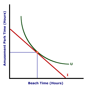
The key in combining what is feasible and what is desirable is to notice that our budget line and indifference curves can go on the same graph since they have the same axes. We know from this that individuals can only reach indifference curves that are in the feasible set (at least least a single point). Getting more would be nice but it's not in the cards. So, since the goal of the consumer is to maximize utility, the choice the consumer makes has to be the one that gives the highest utility for the given budget, which means it's going to have to be on the budget line somewhere.

Because of the other assumptions we make about how indifference curves work, we know that the best or highest indifference curve can't be one that cuts below the budget line anywhere, because that would mean our choice is no better than one that gives us less of both goods than we could get. So the choice of the consumer has to occur where the budget line and indifference curve are tangent (touch at one and only one point). This also yields the interesting result that the slope of the budget line, which is the relative prices and thus represents the trade-off between the two goods in the market, has to be equal to the slope of the indifference curve, which is the marginal rate of substitution and represents the trade-off between the two goods in the mind of the consumer. This makes sense: if apples are $1/lb and oranges $2/lb, but in your mind you'd be willing to swap 3 apples to get an orange, you have incentive to change your behavior: buy fewer apples and more oranges. So the choice of the consumer has to look like the graph on the right.

Once we think of equilibrium this way, we can see that the price of the good, the price of related goods (or what you think the price will be in the future), and your income (or what you think your income will be in the future) will all change the quantity demanded in the ways we've been saying they will with demand curves. The demand curve is derived from the combinations of goods that the consumer views as utility maximizing for various prices, and this relationship shifts when anything else that changes the budget line shifts. Finally, of course, if your preferences (in the form of indifference curves) change, then of course your choice will too.

The last thing we covered this week is that we don't need to know for sure how much utility a choice will give us as long as we can figure out our expected utility. This makes matters a bit more complicated, but it brings up the idea that people tend to dislike taking risks (this skiing guy notwithstanding). Most of us, if given the choice between going home as we are, or risking $50 against somebody else (winner takes home all $100, so $50 extra) on a fair coin flip, we'll just go home. Actually, even if the other guy puts an extra $5 on the table, so we could win bigger than we could lose, we'd still walk away. It's worth something to us to have the guarantee rather than taking the risk.

We actually assumed this was the case last week when we said consumers had diminishing marginal utility. This assumption means that the line representing different chances of winning a high level of utility or a low level is always below the utility function itself. Essentially, expecting to win $200 on average is never going to make us as happy as having $200 for sure. Not only that, but depending on our chances of winning big (where on the line we are), the gamble gives us the same utility as if we were guaranteed a smaller amount of money, say $175. We would actually be willing to pay up to $25 of the expected winnings in order to be guaranteed that we won't lose.

This risk-aversion is what makes insurance companies profitable. You see, all of life involves gambles we can't really get out of--car crashes, house fires, severe illness or injury, you name it--and we are willing to accept a little bit less than we would get on average if only we can be guaranteed the outcome. The insurance company makes an offer: if you win $400, we'll take the money and you'll only get $180 of it; but if you win nothing, we'll still give you $180, and we'll eat the loss. Since we're risk averse, this guaranteed $180 gives us more utility than expecting $200 on average (which gave as much utility as a guaranteed $175). The insurance company knows if it does this a lot, it will bring in about $200 per person and only have to pay out $180. Steady employers can work this way, too: if you did your job freelance you might be able to make more money on average, but your income would go up and down a lot depending on how business is doing this week. If you take a steady job, though, your employer absorbs at least some of the risk, so you're OK making a bit less.

So there you have it. Equilibrium choices, with and without risk. We'll have more to say about risky decision toward the end of the semester. The key idea will be that risk works this way assuming everyone involved is uncertain about the same things. Things get trickier when one side of the market knows something about the outcome that the other doesn't. But that's for another day.

Next week I'm  giving an exam, so no lectern post. I'll have to come up with something fun instead!

Two Links on Teaching

Advice on how college professors should teach from Lee Craig and Craig Newmark. I like some of the suggestions, while others I don't think I buy into. I'll just mention a couple of my favorites here.

Via Lee Craig:

Outlines are good; scripts are bad.

On course evaluations, Lee focuses on what he can control: (1) Were you organized?, (2) Did you treat students professionally?  You cannot control how *effective* you are as a teacher because you cannot control what prejudices students bring to the classroom.

Via Craig Newmark:

For a minute or two every couple of classes raise your voice to almost a yell. This will startle the sleepy students and will entertain the others because it will remind them of Jon Stewart, who they love. Related: schtick is your friend.

One of the most effective ways to build credibility is to demonstrate that you (sometimes) know exactly what the students are thinking. When discussing a difficult bit of material or question, say "You may be wondering [what they're wondering] . . ." or "If you thought the answer was ______, here's a better way to think about it." On the first day of many of my courses, particularly my MBA course, I say, "You may be asking yourself: 'If you're so smart, why aren't you rich?'" Watch the students' eyes widen in surprise as they think, "How did the old guy know I was thinking that?"

I'm interested in what you readers like and dislike about the lists. Are there any of these that all your favorite teachers had in common? Any that you think are actually horrible recommendations?

Dying Majors?

What follows is a response to this article, which describes 10 college majors the author believes are in permanent decline. While I would always advise taking a grain of salt with any opinions about higher education published on a site named 'Online Degree Programs,' I think the idea of education moving away from these areas is interesting enough to comment on. My interpretation is pretty much guided by a single principle: The primary purpose of an undergraduate degree is a signal of innate ability.

Philosophy and the Classics. The article claims the number of people majoring in these areas is down. They don't offer any real data, but do provide some anecdotal evidence. Personally, I find it unlikely that these are permanently shifting down. My reasoning is that most BA degrees from Arts & Science colleges pretty much send the same signal to the potential employers regardless of the major. The ability to think, to read carefully, to do busywork that requires literacy and numeracy--these are the main things employers need to see from an undergraduate degree. Almost no one with a BA uses technical skills learned from the major in a work environment, they're all learned on the job. In this sense, Philosophy and Classics are just two flavors of the same signaling device, along with Political Science, Mathematics, English, and of course Economics. The only way these majors are actually on their way out is if students are look for more vocational training in their college curriculum. Personally, I'd like to see more people in vocational training than in traditional college studies, but I doubt this is a long run trend. More likely the relatively unimpressive economic performance of the last decade has inclined people toward more targeted skill sets. If the economy returns to the average growth we saw from 1950-2000 (and we have no reason to think it won't), I suspect this trend will reverse itself.

<insert people group here> Studies and Social Work. I'm honestly not surprised American Studies (as the article calls it) are on their way out, despite my previous statement about the BA as a generic signal. The key difference is that programs focusing on specific people groups are narrowly focused enough that they don't necessarily represent utilization of the broad skill sets of more conventional BA's, but they're still vague enough that not everyone knows what skills do get utilized (and this probably varies depending on which program at what school we're talking about). I think the article makes a good point: a literature or history degree sends a more easily interpreted signal, so these departments seem likely to absorb faculty and students from American Studies (those that don't fall victim to the recession, that is). Social Work is a bit more surprising, but much that they do could be absorbed by Psychology departments, and that degree is broad enough to appeal that if social work doesn't turn out that great (or the low pay gets annoying), there are other job prospects.

Journalism. Given the recent construction of the new Temple of Apollo Journalism College building on my own campus, I find this one a bit hard to believe. It's true that newspapers are a dying breed. Free content news sources that make use of internet technology are primarily going to replace the one or two print editions per day/week that make up the newspaper business model. Even TV news is probably going to be supplanted by sources that provide information online as it develops. But there will always be people willing to pay for information condensation and filtering (and perhaps more importantly, there will always be those who want to advertise to those who want this service). I suspect that journalism schools will shift the media tools they teach--newsprint is out and blogging is in. But as the technology makes getting information out there easier, the skills needed to attract a readership and keep them interested over time will probably have an increased demand, not a reduced. People are going to need a way to signal that they're not just armchair reporters.

Foreign Languages and Humanities. Foreign language is sort of a mislabeled degree in the first place, since the goal is always to learn not just the language of a culture but their history, customs, and common modes of thinking as well. For English speakers, this has long been largely a matter of recreation, since most other cultures are willing to adapt to the English speaking world in order to conduct business. And in as much as they are known to be matters of recreation, they don't send as good a signal as many other BAs. However, the next 20 years could easily see the rise of China and India to rival the current big 3 economic powers (US, EU, and Japan). For that matter, recent events have suggested that the staying power of the EU is not what we previously thought, so we could see a massive leveling of the playing field across eastern and western hemispheres. If this is the case, then I think we'll see two groups of people doing a lot of studying in foreign languages and humanities (or letters as it's called here): a renewal of recreational education as international trade leads to renewed growth, and people shooting for influential positions in multinational corporations. That's right, I think trade contracts in the mid-21st century are going to depend a lot on corporations playing to local loyalties in a way not yet seen. I see a lot more future tension between globalization and xenophobia, and familiarity with the national personality might be the signal a corporate vice president needs to tip the scales in their favor.

These beliefs could be way off base. I don't think online degree programs will ever make up a large share of the higher ed market, much less replace current universities (although I think current universities will absorb a lot of techniques from these programs). So take my predictions with a grain of salt, and we'll see how I did in 2030.